Step-by-Step Guide: Applying Date-Based Conditional Formatting in Microsoft Excel

Quick Links

Conditional formatting is a terrific feature for automatically applying highlights or font formats to cells. If you have an Excel spreadsheet that contains dates, you can use this feature to make certain dates stand out and easy to spot.

Whether you want to format past due dates for household bills or upcoming dates for a project plan, conditional formatting has you covered with both simple and custom options. Just set up the rule and watch your dates pop off of the sheet.

Apply a Quick Conditional Formatting Date Rule

If you want to create a quick and easy conditional formatting rule , this is a convenient way to go. Open the sheet, select the cells you want to format, and head to the Home tab.

In the Styles section of the ribbon, click the drop-down arrow for Conditional Formatting. Move your cursor to Highlight Cell Rules and choose “A Date Occurring” in the pop-out menu.

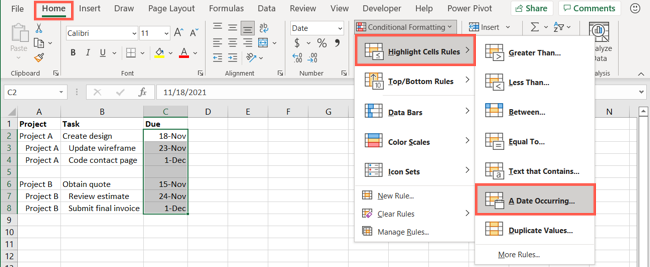
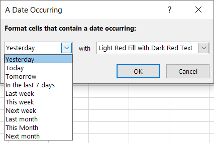
A small window appears for you to set up your rule. Use the drop-down list on the left to choose when the dates occur. You can pick from options like yesterday, tomorrow, last week, and next month.

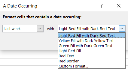
In the drop-down list on the right, pick the formatting you’d like to use. You can select from formats like a light red fill, yellow fill with dark yellow text, and a red border.

When you finish, click “OK” to apply the conditional formatting rule to the selected cells.

Create a Custom Conditional Formatting Date Rule

Maybe you’re not fond of the formatting choices available when creating the quick rule above. You can set up custom formatting instead. This allows you to format the cells most any way you like, including using more than one format for the cells like a specific font, border, and fill color.

You can create a custom format two ways in Excel.

Custom Format Method One

The first way is to start with the same setup as above. In the pop-up window where you create the rule, use the format drop-down box to pick “Custom Format.”

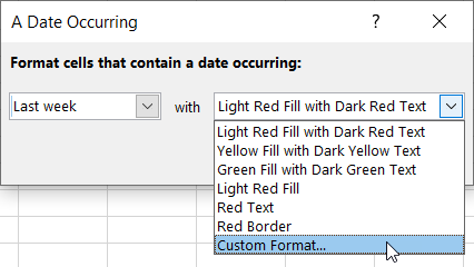
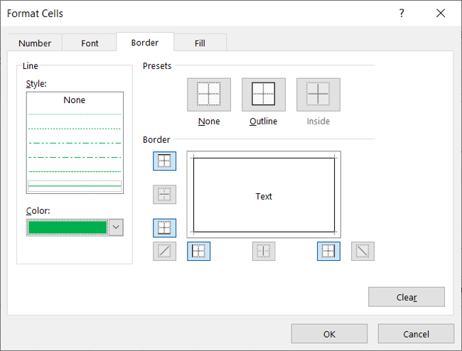
When the Format Cells window opens, use the tabs at the top for Font, Border, and Fill to create your custom format. Click “OK” when you finish.

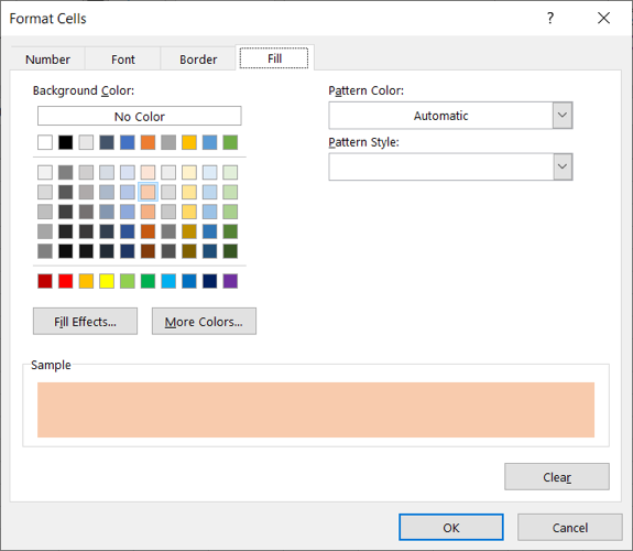
You’ll see the custom format applied to the cells. Click “OK” in the small window to save the change.

Custom Format Method Two

The second way to create a custom conditional formatting rule is to use the New Formatting Rule feature.

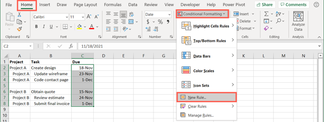
Select the cells you want to format and go to the Home tab. Click the Conditional Formatting arrow and choose “New Rule.”

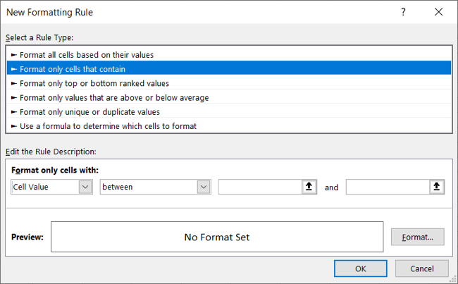
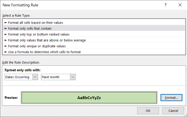
In the New Formatting Rule window, choose “Format Only Cells That Contain” in the Select a Rule Type section.

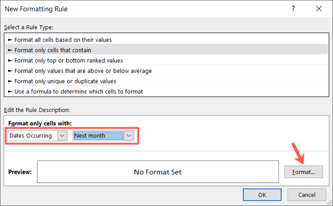
At the bottom of the window, select “Dates Occurring” in the drop-down box on the left and choose the timeframe for the date to the right. Then, click “Format.”

You’ll see the same Format Cells box as above where you can use the Font, Border, and Fill tabs to create the custom format. When you finish, click “OK.”

The options you pick appear in the New Formatting Rule window as a preview. If you’re happy with the format, click “OK” to save the rule.

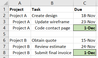
You’ll then see your cells updated with your custom format.

Click here

Notes on Conditional Formatting Based on Date in Excel

With a conditional formatting rule in place, it applies to any edits you make to the dates in the cells. For example, say you formatted dates for next week. If you change any of the dates to yesterday, the formatting automatically disappears.

You can set up more than one rule for the same cells. Maybe you want to see all dates this month with a red font and all those next month with a green font. You would simply follow the same steps to create each rule and adjust the formatting accordingly.

For things like bills or tasks that are past their due dates or those you have coming up soon, you can spot them quickly with conditional formatting in Excel .

Win Solutions

Step-by-Step Guide: Applying Date-Based Conditional Formatting in Microsoft Excel