Why I Rely on Conditional Formatting for Enhanced Spreadsheet Analysis

Quick Links

• How Do You Access the Conditional Formatting Tool?
• Conditional Formatting Can Highlight Certain Values
• Conditional Formatting Works With Changing Data
• You Can Compare Data Easily
• Things to Note

Manually highlighting values in large data sets can be both time-consuming and error-prone, especially if your data is likely to change over time. With that in mind, using conditional formatting can help eliminate these two hurdles.

Conditional formatting formats a cell or a range of cells based on conditions you have applied. In the examples below, I will show you some everyday uses of this incredibly useful tool, so you can let Excel do the hard work for you.

Click here

How Do You Access the Conditional Formatting Tool?

To access the conditional formatting tool, highlight the cell or cells you want to format, and in the Home tab on the ribbon, click “Conditional Formatting” in the Styles group. From there, you’ll see the many different options available.

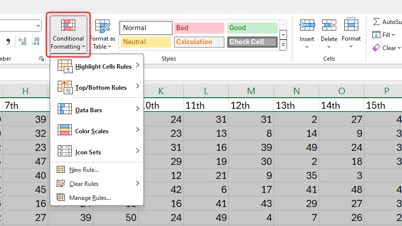
I’m not going to run through every use of conditional formatting, as there are hundreds! Instead, I want to share with you a few practical uses that you can apply to everyday tasks.

Conditional Formatting Can Highlight Certain Values

Among its many uses, Excel is best known for its ability to present and organize data for you to use and analyze. To make the analysis process much easier, you can use conditional formatting to highlight cells containing certain values, unique or duplicated cells, highest and lowest values within a data set, and in many other similar scenarios.

Highlighting Cells Containing Certain Values

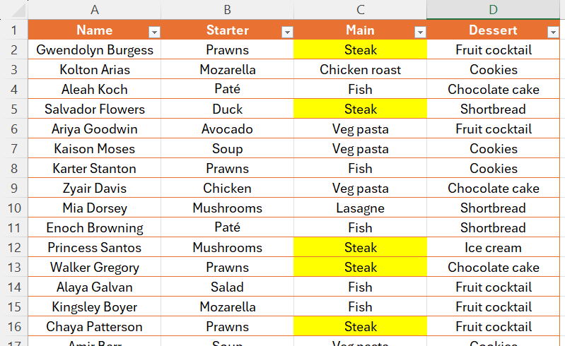
Let’s say you’re organizing a party, and you’ve taken everybody’s food orders. You now want Excel to highlight every steak order, as you need to ask the guests how they like it cooked.

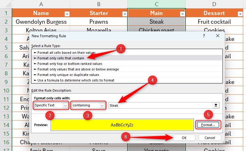
First, select the data that you’re applying the condition to—in this case, it’s the whole of column C. Then, in the Conditional Formatting drop-down menu, click “New Rule.”

In the dialog box, click “Format Only Cells That Contain,” and in the first drop-down option, select “Specific Text.” Make sure you click “Containing” in the next drop-down box, but note the other options that you can also use at this stage. Then, in the empty field box, type the text you want to highlight within your selected cells—in our case, it’s “Steak”—and then create the formatting you want for these cells by clicking “Format.” Once you’re done, click “OK.”

Now, all cells containing “Steak” will be highlighted in yellow.

Highlighting Unique or Duplicated Cells

You can use conditional formatting to easily identify duplicates or anomalies in a data set. This is a really effective way of efficiently cleaning up your spreadsheet. I use this tool all the time on my vacation packing list. As I’m always adding to it and accessing it both on my computer and on the move through OneDrive , I sometimes accidentally add items that are already there.

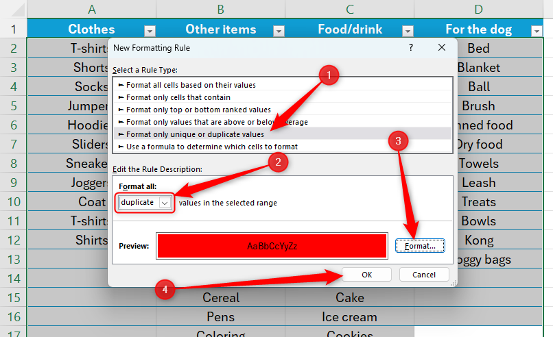
To automatically highlight duplicated cells , select the relevant data, and in the Conditional Formatting drop-down menu, click “New Rule.”

In the resultant dialog box, click “Format Only Unique Or Duplicate Values,” and in the drop-down, select “Duplicate.” Define the formatting you want for these cells by clicking “Format.” Once you’re done, click “OK.”

This is how my vacation packing list looks when I apply this tool.

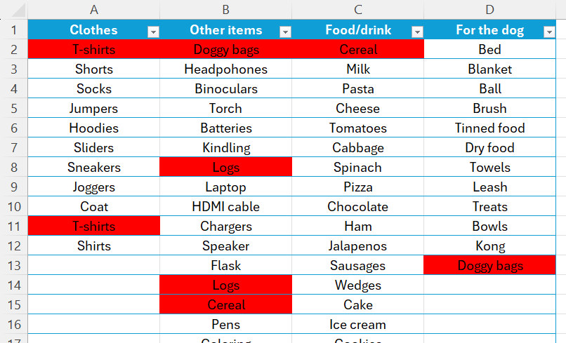
I can now go and delete one of each item that is duplicated. And because the conditional formatting is adaptable, as soon as I delete a duplicate, the other also loses its formatting (as it’s no longer a duplicate). As a result, I’ll end up with a nice, tidy spreadsheet.

You can also do the same with unique cells—that is, cells that contain data different to the rest of the array. Simply click “Unique” instead of “Duplicate” in the relevant drop-down menu.

Highlighting the Highest and Lowest Values

As an avid football fan, I like to rate players based on their performance in each game, and then easily see who has played consistently well. To do this, I make Excel automatically highlight the highest two ratings for each game.

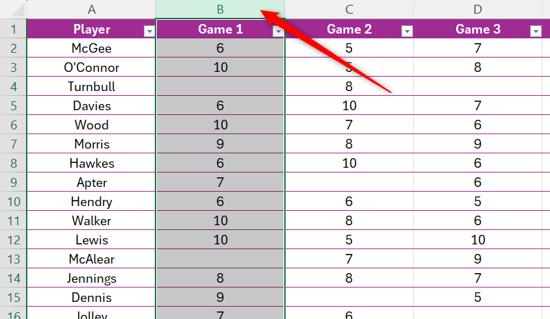
First, select the data range you want to evaluate. In my case, it will be the first column containing data. I don’t want to select all the data in my table, as then that will highlight the highest two ratings across all games, whereas I want to do this for each game individually.

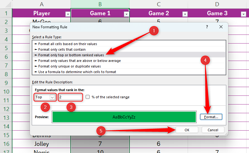
Then, in the Conditional Formatting menu, click “New Rule.” In the dialog box, click “Format Only Top Or Bottom Ranked Values,” and in the drop-down option, select “Top” (or click “Bottom” if you want to highlight the lowest values). Next, in the number field, type the parameters of your conditions. For example, if you click “1”, this will highlight the single top value in your data. Also check the “%” box if you want to state your parameters as a percentage. Create the formatting you want for these cells, and once you’re done, click “OK.”

This is how my sheet will look. Notice how five scores have been highlighted, as more than two people achieved the high-score parameter I set in my rule.

Next, you should use the Format Painter to apply the same conditions to the next column, and then change the formatting of the values meeting your criteria, so that it’s distinguishable from the first column.

Conditional Formatting Works With Changing Data

In the first section, we formatted cells containing a set value, but Excel also lets you easily change the parameters for formatting your cells without having to amend the rules.

For example, let’s assume we have various household jobs that need to be completed, and we’ve assigned each job to a family member on each day. We now want to see all the jobs that a certain family member has been assigned.

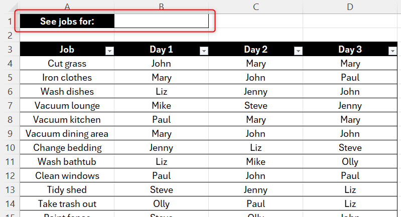
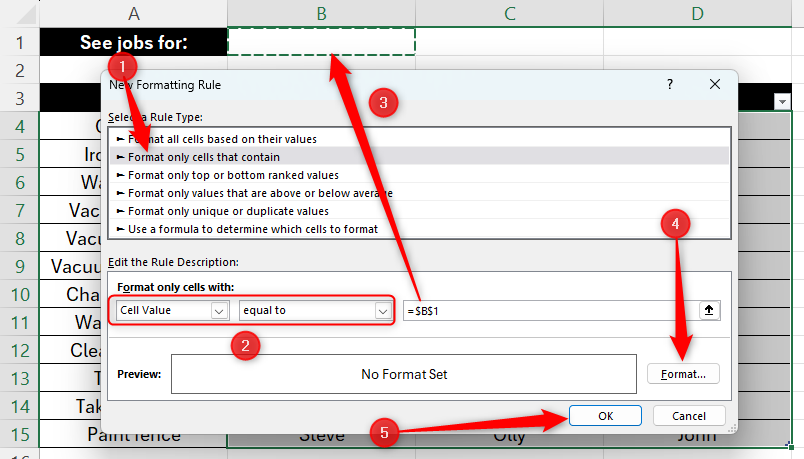
To do this, first select all the data you want to search. Then, in the Conditional Formatting menu, click “New Rule.” In the dialog box, click “Format Only Cells That Contain,” and in the first drop-down option, select “Cell Value.” Next, in the second drop-down field, click “Equal To.” Then, click the text field, before clicking the cell that you’re going to use as your variable parameter. In our case, that’s B1. Finally, create the formatting you want for these cells, and click “OK.”

Click here

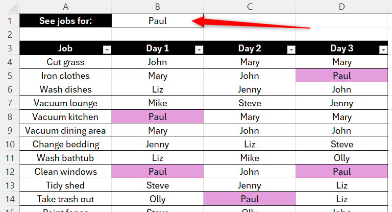
Then, in the cell you selected in your conditional formatting rule, type a word or number that matches some of the data in your table to see each case of that word or number being highlighted.

You could also choose the variable value from a drop-down list you create in Excel .

You Can Compare Data Easily

So far, I’ve talked about how conditional formatting can help you to identify certain values within a set of data. However, conditional formatting is equally useful for comparing numbers within a range .

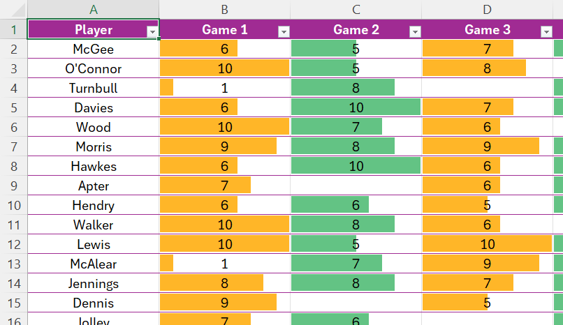
Going back to the football player ratings from earlier, rather than highlighting the highest or lowest values, let’s compare how all the players performed.

First, select the data you want to use. In our case, it’s the ratings from the first game in column B. Then, in the Conditional Formatting drop-down, choose from the three following options:

• Data Bars (see screenshot below)—This partly fills each cell depending on the value compared to the others in the range. The cells containing the highest value will be fully filled, and the cells with the lowest value will be fractionally filled.
• Color Scales—This colors the cells in a gradient depending on the values they contain.
• Icon Sets—This adds different icons depending on the cell values.

Things to Note

If you do, indeed, get the conditional formatting bug and find that you use it in most of your spreadsheets as I do, then there are a few small things to note.

• The more conditional formatting you include (or the larger your data set containing conditional formatting), the slower things might become in your spreadsheet. This is because Excel has to apply the conditions to each cell individually, and if you have lots of rules, this can take some time. There’s no issue with this if you’re willing to wait, but if you’re looking to work speedily, it’s worth limiting its use.
• Be careful with overlapping rules, especially if you inadvertently apply contradicting conditions to a cell. Make sure you know exactly where your existing formatting rules are before adding new ones.
• Adding rows and columns or moving things around where conditional formatting is already in place can cause problems. As with the previous point, make sure you know where you have already placed some rules, and double-check that they are where you want them to be after making changes to your sheet’s layout.

In the Conditional Formatting drop-down list, you can also manage the rules applied to your sheet , and you can also clear rules from selected cells, the entire sheet, or a table.

Also read: